41 conditional formatting data labels excel
Value-based conditional formats - Data Visualizations using Conditional ... He wants to do this using conditional formatting. Let's start by moving our map out of the way so we can actually see the cells behind. We've actually labeled each of the cells. What our conditional formatting needs to do is to check if the label above the cell we want to highlight is equal to the selection, then we're going to change the color. Change the format of data labels in a chart To get there, after adding your data labels, select the data label to format, and then click Chart Elements > Data Labels > More Options. To go to the appropriate area, click one of the four icons ( Fill & Line, Effects, Size & Properties ( Layout & Properties in Outlook or Word), or Label Options) shown here.
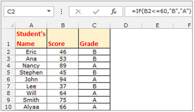
How To Use Conditional Formatting in Excel in 5 Steps 4. Select an option from the drop-down menu. Once you select the "Conditional Formatting" button, Excel displays several options, starting with "Highlight Cells Rules" and ending with "Manage Rules." Selecting one option from the first five allows you to develop rules based on the option you choose.

Conditional formatting data labels excel
r/excel - Is it possible to conditionally format Data Labels on a ... By data labels I mean the actual data numbers that appear above the line that's plotted, to avoid confusion. I remember seeing somewhere that, for example, if a negative number is plotted then colour RED is used to colour that data label and BLUE if it's positive via the use of Custom Cell Formatting option. Many thanks 3 comments 81% Upvoted How to change chart axis labels' font color and size in Excel? Sometimes, you may want to change labels' font color by positive/negative/ in an axis in chart. You can get it done with conditional formatting easily as follows: 1. Right click the axis you will change labels by positive/negative/0, and select the Format Axis from right-clicking menu. 2. Conditional Formatting in Excel - a Beginner's Guide - GoSkills.com Click Conditional Formatting, then select Icon Set to choose from various shapes to help label your data. For this example, let's use the arrow icon set to show whether our highlighted data, the Variance column, has increased or decreased. Now, you'll see that the data has arrow icons accompanying their values in the cells.
Conditional formatting data labels excel. How to create a chart with conditional formatting in Excel? - ExtendOffice Add three columns right to the source data as below screenshot shown: (1) Name the first column as >90, type the formula =IF (B2>90,B2,0) in the first blank cell of this column, and then drag the AutoFill Handle to the whole column; How to Create Excel Charts (Column or Bar) with Conditional Formatting ... Conditional formatting is the practice of assigning custom formatting to Excel cells—color, font, etc.—based on the specified criteria (conditions). The feature helps in analyzing data, finding statistically significant values, and identifying patterns within a given dataset. Progress Doughnut Chart with Conditional Formatting in Excel Mar 23, 2017 · Great question! The Excel Web App does not support those text box shapes yet. We can use the built-in data labels for the chart instead. The label for the Remainder bar can be deleted by left clicking on the label twice, then pressing the delete key. That just leaves the data label for the actual progress amount. Here is a screenshot. Changing the Color of a Data Label using IF Statement 1) Click on the data labels to highlight all the data labels, 2) Right-Click and select Format Data Labels, 3) Click on Number, 4) Go to the Format Code field *adapt the following to your needs* 5) [green] [>29]#.00; [<30] [Color 53]#.00 Click to expand... Hi Jawnne, I hope you're still lurking about on here.
Conditional Formatting For Blank Cells | (Examples and Excel ... Always use limited data to deal with and apply bigger conditional formatting to avoid excel getting freeze. Recommended Articles. This has been a guide to Conditional Formatting for Blank Cells. Here we discuss how to apply Conditional formatting for blank cells along with practical examples and a downloadable excel template. Excel conditional formatting Icon Sets, Data Bars and Color Scales Excel conditional formatting icon sets will help you visually represent your data with arrows, shapes, check marks, flags, rating starts and other objects. You apply the icon sets to your data by clicking Conditional Formatting > Icon Sets, and the icons appear inside selected cells straight away. In the screenshot above, you can see a table ... Excel Data Analysis - Conditional Formatting - tutorialspoint.com Follow the steps to conditionally format cells − Select the range to be conditionally formatted. Click Conditional Formatting in the Styles group under Home tab. Click Highlight Cells Rules from the drop-down menu. Click Greater Than and specify >750. Choose green color. Click Less Than and specify < 500. Choose red color. Customize the horizontal axis labels - Microsoft Excel 365 2.2. In the Edit Series dialog box: . For the scatter chart, in the Series X values field, type the same data as for the other data series to see the same values on the horizontal axis.; In the Series values or Series Y values box, type the constant values equal to the minimal visible value on your chart as many times as many labels you want to see on the chart.
Creating Conditional Data Labels in Excel Charts - YouTube We can make labels appear on our charts that don't have to do with the raw numbers that built the chart - and we can make them show up or not based on whatever conditions we want. In this tutorial,... r/excel - Conditional Label Formatting in Excel Charts level 1. · 11m. 247. Just a note: conditional formatting refers to the highlighting/border effects that can be applied to cells based on their values (or formula). Your dropdown list was created using data validation. Anyways, to your issue: a chart will display the axes labels and data labels (two different things here) based on the ... How-to Make Conditional Data Labels for an Excel Dashboard Checkout the Step-by-Step Tutorial here: on How to conditionally hide and unhide data labels ... Conditional formatting chart data labels? - Excel Help Forum The easy way to conditionally format these labels is use two series. Use something like =IF($E2=1,0,NA()) for the series that has red labels and =IF(#E2=1,NA(),0) for the series that has unformatted labels. Jon Peltier Register To Reply Similar Threads Conditional Number Formatting Not Working for Chart Value Labels
How to Create a Risk Heatmap in Excel - Part 2 - Risk Management Guru
Custom Data Labels with Colors and Symbols in Excel Charts - [How To ... Step 4: Select the data in column C and hit Ctrl+1 to invoke format cell dialogue box. From left click custom and have your cursor in the type field and follow these steps: Press and Hold ALT key on the keyboard and on the Numpad hit 3 and 0 keys. Let go the ALT key and you will see that upward arrow is inserted.

HIGHLIGHT DUPLICATE VALUE IN EXCEL - Data analysis
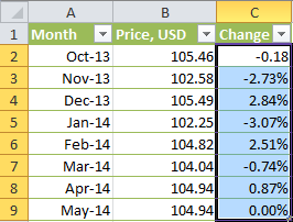
Excel bar chart with conditional formatting based on MoM change Click on any bar and press Ctrl+1 to make the Format Data Series task pane appear if it is not already showing. In the Series Options section, set the Gap Width to 50% to give the bars more presence and set the Series Overlap to 100%. Use the chart skittle (the "+" sign to the right of the chart) to remove the legend and gridlines.
How to use conditional formatting in Excel
Conditional Formatting with Data Validation - Microsoft Tech Community For example, if A2=Value, B2= Value, and C2 is blank, I would like to have C2 turn red. A2,B2, and C2 all have a list range for the Data Validation. For the conditional formatting, I have only put the range to apply to as column C. The conditional formatting is not turning cells red as needed. I am not sure what the issue is.

How to Create Multi-Category Chart in Excel - Excel Board
Microsoft Excel conditional number formatting Sep 17, 2019 · Next, I would apply conditional formatting number formatting where the cell value is greater than one so that numbers greater than a million could be displayed to the nearest 0.1m, numbers less than a million but greater than or equal to 1,000 could be displayed to the nearest 0.00k and numbers lower than 1,000 (but necessarily greater than one ...
HOW TO COPY CONDITIONAL FORMATTING IN EXCEL? - GyanKosh | Learning Made Easy
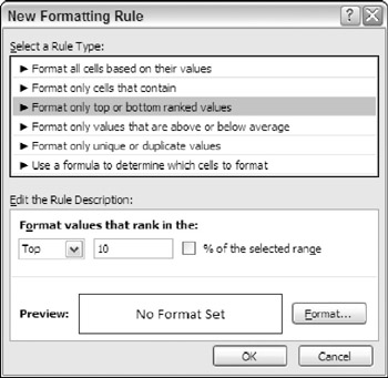
Conditional formatting with formulas (10 examples) | Exceljet You can create a formula-based conditional formatting rule in four easy steps: 1. Select the cells you want to format. 2. Create a conditional formatting rule, and select the Formula option 3. Enter a formula that returns TRUE or FALSE. 4. Set formatting options and save the rule.

How To Use Conditional Formatting in Excel - YouTube
How to Change Excel Chart Data Labels to Custom Values? May 05, 2010 · Now, click on any data label. This will select “all” data labels. Now click once again. At this point excel will select only one data label. Go to Formula bar, press = and point to the cell where the data label for that chart data point is defined. Repeat the process for all other data labels, one after another. See the screencast.

How to use Conditional Formatting in Excel? - GeeksforGeeks
Format Data Labels in Excel- Instructions - TeachUcomp, Inc. To format data labels in Excel, choose the set of data labels to format. To do this, click the "Format" tab within the "Chart Tools" contextual tab in the Ribbon. Then select the data labels to format from the "Chart Elements" drop-down in the "Current Selection" button group.

How to Create a MS Excel Pivot Table – An Introduction | SIMPLE TAX INDIA
Excel tutorial: How to add a conditional formatting key Let's go one step further, and color-code our key to match the table, using the same conditional formatting. To make this change, we need to edit each rule again, and add the address for the appropriate cell in the key. For each rule, we click into the address, add a comma, then select the appropriate cell in the key.

Advanced Graphs Using Excel : Heat map plot in excel using conditional formatting
Conditional formatting for chart axes - Microsoft Excel 365 You can't apply conditional formatting - Excel ignores the custom conditional formatting for such axes: For the horizontal (Category) axis labels in line, column, and area charts, For the vertical (Value) axis labels in a bar chart. So, the standard conditional formatting can be applied for both axes just for scatter plots.
How to Use of Conditional Formatting in Microsoft Excel
How to Add Data Bars in Excel? - EDUCBA How to Add Data Bars in Excel? Data Bars in Excel. Data Bars in Excel is the combination of Data and Bar Chart inside the cell, which shows the percentage of selected data or where the selected value rests on the bars inside the cell. Data bar can be accessed from the Home menu ribbon’s Conditional formatting option’ drop-down list.

How to Create Multi-Category Chart in Excel - Excel Board
How to do conditional formatting of a label in Excel VBA The TEXT worksheet function seems to respect the format you initially specified and you can use it in your VBA by virtue of Application.WorksheetFunction.. Application.WorksheetFunction.Text(812, "[>=1000000] $#,##0.0,,""M"";[>0] $#,##0.0, ""K"";General") The VBA reference for FORMAT doesn't cover conditional number formatting but it does have a number formatting section, so I expect ...
Chapter 19: Conditional Formatting and Data Validation | Excel 2007 Formulas (Mr. Spreadsheets ...
Custom Chart Data Labels In Excel With Formulas - How To Excel At Excel Select the chart label you want to change. In the formula-bar hit = (equals), select the cell reference containing your chart label's data. In this case, the first label is in cell E2. Finally, repeat for all your chart laebls. If you are looking for a way to add custom data labels on your Excel chart, then this blog post is perfect for you.
Conditional Formatting of Excel Chart Data Labels – Neil McNiven
Excel Conditional Formatting not functioning correctly after ... Jan 10, 2018 · Everything works fine, formatting changes according to changes in the data! Now I copy a range of sheet A to sheet B using VBA, that works OK. However: in sheet B the conditional formatting of these cells is not working correctly anymore: > cells using 'format only cells that contain' work correct! formatting changes correctly when data changes

How to Create Multi-Category Chart in Excel - Excel Board
Excel Conditional Formatting Data Bars - Contextures Excel Tips On the Ribbon, click the Home tab. In the Styles group, click Conditional Formatting, and then click Manage Rules. In the list of rules, click your Data Bar rule. Click the Edit Rule button, to open the Edit Formatting Rule dialog box. In the second section -- Edit the Rule Description -- add a check mark to Show Bar Only.
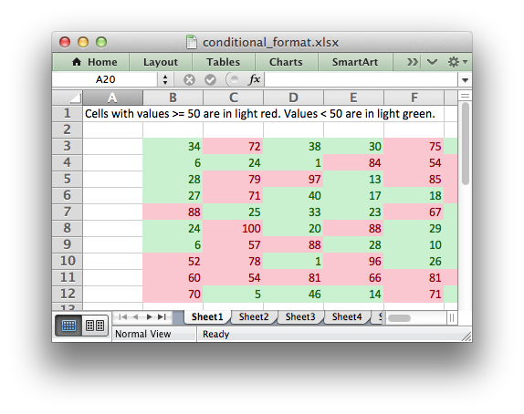
Working with Conditional Formatting — XlsxWriter Documentation
How to Apply Conditional Formatting to Pivot Tables - Excel ... Dec 12, 2018 · Conditional Formatting can change the font, fill, and border colors of cells. It can also add icons and data bars to the cells. The formatting will also be applied when the values of cells change. This is great for interactive pivot tables where the values might change based on a filter or slicer. How to Setup Conditional Formatting for Pivot ...
Daftar Tutorial Macro / VBA Excel
Use conditional formatting to highlight information Conditional formatting can help make patterns and trends in your data more apparent. To use it, you create rules that determine the format of cells based on their values, such as the following monthly temperature data with cell colors tied to cell values.

excel - Save applied formats of conditional formatting - Stack Overflow
VBA Conditional Formatting of Charts by Value and Label The first series of the active chart is defined as the series we are formatting. The category labels (XValues) and values (Values) are put into arrays, also for ease of processing. The code then looks at each point's value and label, to determine which cell has the desired formatting. The rows and columns are looped starting at 2, since the ...
Post a Comment for "41 conditional formatting data labels excel"